Interactive spike sorting

This tutorial shows the basic procedure of detecting, sorting, and exporting the spike data with the SpikeSort software. Here, we use the built-in component based command-line interface SpikeBeans, which is very easy to use.

You will also find the information on how to adjust the provided scripts for your needs.

Note

The procedure described in this tutorial can also be implemented using the SpikeSort’s methods directly (see Using low-level interface).

The procedure consists of three steps:

• Reading the data
• Spike sorting
• Exporting results

1. Reading the data

Before you can start spike sorting you have to load data with raw extracellular recordings. Such data can be obtained from microelectrodes, tetrodes or shank electrodes. SpikeSort currently supports data saved in custom binary and HDF5 format but new formats can be easily added.

To start with, you can download a sample data file.

This hierarchical file is organized as following:

/subject/session/electrodeid

For example, data from electrode el1 recorded in session session01 of subject SubjectA can be found under /SubjectA/session01/el1

I will assume that you downloaded this file and saved it to data directory.

The fastest way prepare the data, is to use the provided script cluster_beans.py which can be found in the SpikeSort/examples/sorting/ directory. By default, the script is configured and ready to use with the tutorial data. For now, we’ll use the unmodified version. However, you can find the detailed information on how to adapt the script for your needs at the end of this tutorial.

Before you run the script, create the environment variable called DATAPATH which points to the folder where the data is located. On UNIX-based systems, it can be added from the terminal as follows:

$ export DATAPATH='where/your/data/is/located'

Then, just fire it up from the python shell in the interactive mode:

$ python -i cluster_beans.py

or, alternatively, within the ipython interactive shell:

$ ipython cluster_beans.py

Now everything is ready to start sorting the spikes.

Note

IPython is an enhanced Python interpreter that provides high-level editting functions, such as tab-completion, call-tips, advanced command history and documentation access. It is the recommended way of working with SpikeSort.

2. Spike sorting

A. Visualizing the data

To provide some useful data visualization tools, the cluster_beans.py creates four plotting objects:

• browser - the Spike Browser
• plot1 - feature space viewer
• plot2 - spike waveshape viewer
• legend - legend of the colour code used in all plots

In order to see the output of such an object, just call its show() method, e.g.:

>>> browser.show()

Each plotting component is described in detail below.

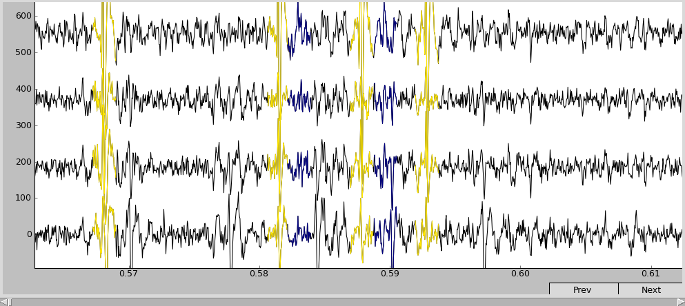
Spike Browser

The four horizontal black curves are the [filtered] voltage traces recorded from different channels (channel 0 at the bottom and 3 at the top) of the electrode el1 (can be changed in the script). The color segments are the detected spikes’ waveshapes. The correspondence between color and cell index can be found in the legend.

Use the “+” and “-” keys to scale the vertical axis, and the “Prev” and “Next” buttons to navigate across the temporal axis. Now it looks more comprehensible:

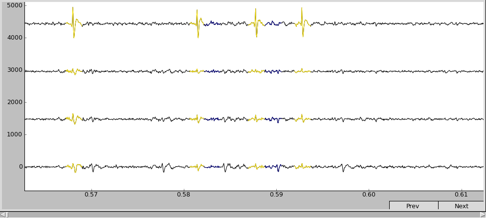
Spike browser after scale adjustment.

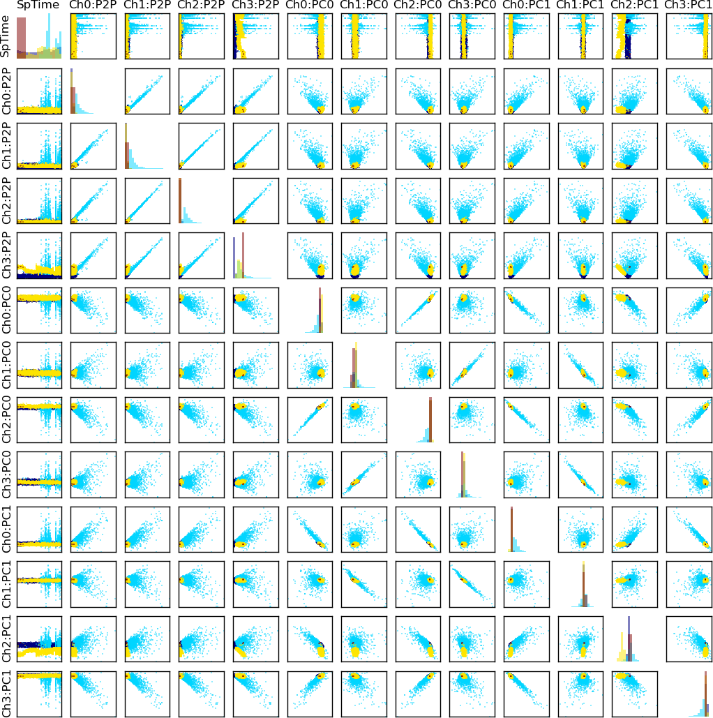
Feature plot

To sort the spikes, some characteristic features that may be used to differentiate between the waveshapes have been calculated (e.g. peak-to-peak amplitude, projections on the principal components).

To help the user identify the features, all features have short labels. For example, feature Ch0:P2P denotes peak-to-peak amplitude in contact (channel) 0.

The Feature space viewer plots the spikes’ projections in the feature space (pair-wise 2D plots) and 1D projection histograms for each feature (on the diagonal). The plot is symmetric - the upper triangle is the same as the lower.

Note

Depending on how many features are viewed, the subplots may be too small. To zoom in/out the subplot, target it with the mouse and press the “z” key.

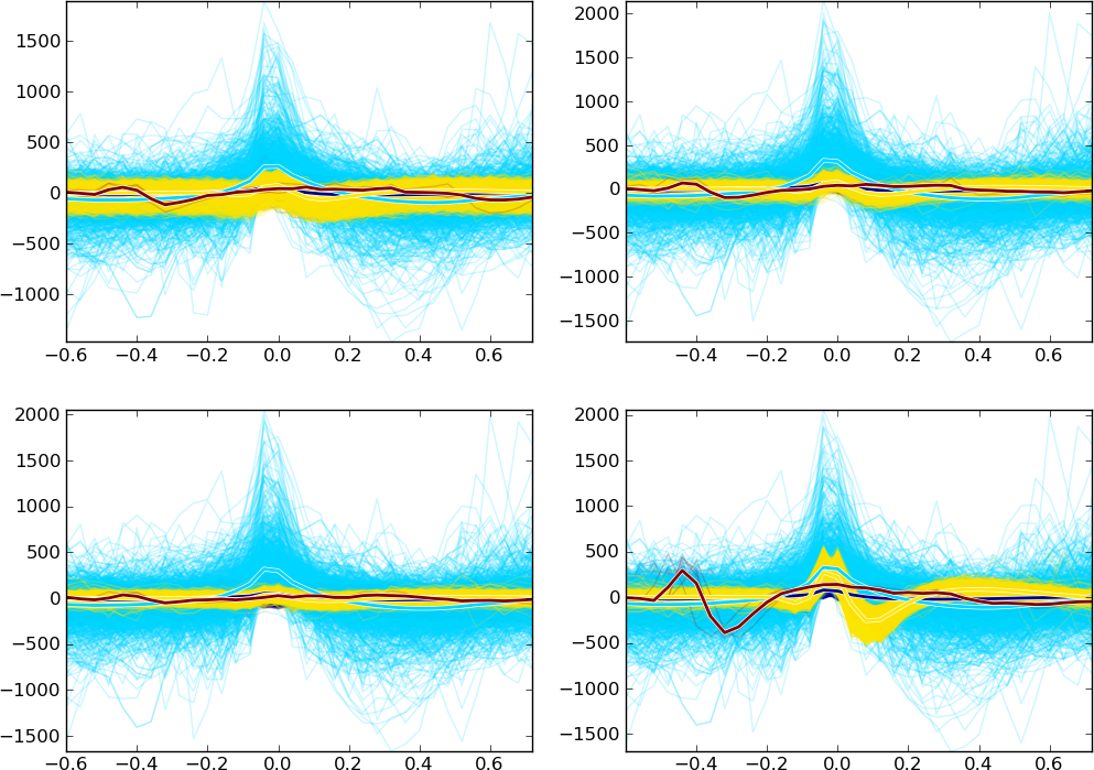
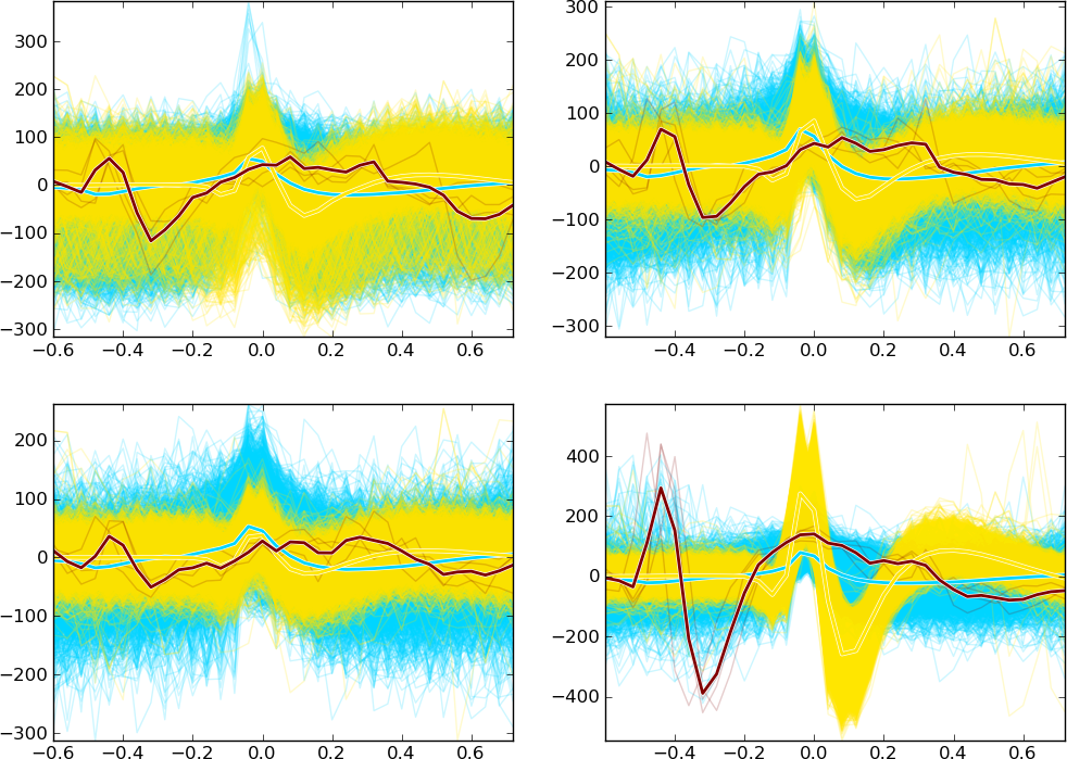
Spike waveshape plot

This component plots the aligned and overlapped spike waveshapes. The spikes recorded from different channels are shown in different subplots arranged from left to right and from top to bottom.

You can also zoom the subplots here as in the Feature space viewer.

Legend

For the convenience, the legend is plotted in a separate figure.

B. Managing the spikes

The aim of the spike sorting is to differentiate one or several cells’ spikes from each other and from other activity (such as background noise or stimulus artifacts). This can be partially done by the automatic clustering in the feature space. However, for the reliable results, some manual manipulations are needed and the best settings have to be identified using trial-and-error procedure. It usually involves removing/merging cells (clusters), reclustering the data, and changing the spike detection threshold.

Before we proceed, it will be convenient to create some aliases:

>>> ca = base.features['LabelSource']         # points to the ClusterAnalyzer
>>> sd = base.features['SpikeMarkerSource']   # points to the SpikeDetector

Note

SpikeSort beans interface consists of independent components each performing one step of spike sorting. base.features is a container with these components. The keys in this container (LabelSource and SpikeMarkerSource) describe the functionality that the components provide: LabelSource provides cluster labels and SpikeMarkerSource provides the times of detected spike events. In this example we search for the components by their functions.

Looking at the spike waveshapes, one might find, that the blue “Cell 2” (in your case, it may have different index and/or coloring since the clustering algorithm uses random initial state) is most probably not really a cell, but some noise. Thus, it is not interesting and we want to remove it.

To remove one or more cells (i.e. clusters), you have to look up their id’s in the legend and then pass them as arguments to the ca.delete_cells() function:

>>> ca.delete_cells(2)

After we got rid of the unnesessaey stuff, the waveshape plot looks as follows:

All the deleted “spikes” are now assigned the id 0, which can be considered as a trash.

Sometimes the clustering algorithm splits one cell into two clusters. In such cases it is convenient to merge them back into a single cell. In our example, there is no need to merge anything. However, cells 1 and 4 (blue and brown) also look like trash, so let’s merge them (just as a practice) and delete afterwards.

The merging procedure is similar to deletion - ca.merge_cells() function takes as arguments IDs of all cells to be merged into one group:

>>> ca.merge_cells(1,4)     # after merging, they form a cell with index 1
>>> ca.delete_cells(1)      # removing the cell 1

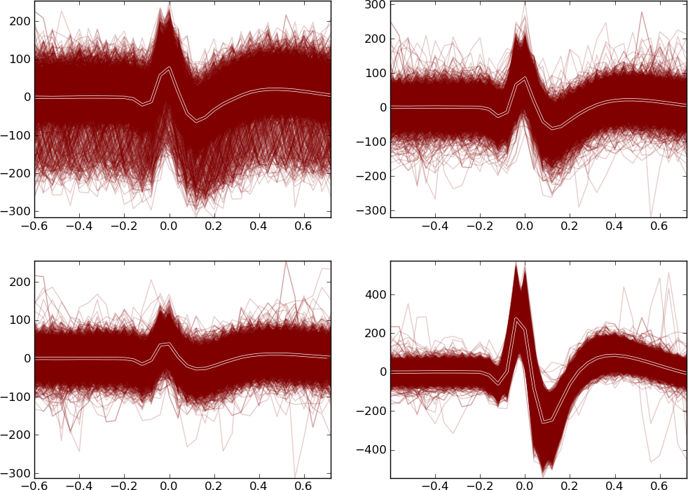
Note that the new cell has an ID of one: the new cluster takes the lowest of the IDs of merged clusters. Now, only the cluster with real spikes is left (brown):

Sometimes, we need to break (recluster) the cluster into two or more (again, because of the incorrect clustering).

To do so, use the ca.recluster() function:

>>> ca.recluster(1, 'gmm', 2)

where the arguments are: cell to recluster, clustering algorithm, and the number of new clusters.

Note

There are several automatic, semi-automatic and manual methods for clustering. Their performance and accuracy depends to large degree on a particular dataset and recording setup. In SpikeSort you can choose from several available methods, whose names are given as the first argument of spike_sort.cluster.cluster() method. The ‘gmm’ shortcut used in this example, means the Gaussian Mixture Model algorithm

In practice, it may happen that the threshold used during the spike detection is too high to detect some important activity or too low to leave the noise out. In this case you can easily change it (as well as any other SpikeDetector property) adjusting the corresponding SpikeDetector property:

>>> sd.threshold = 90
>>> sd.update()

The update() method informs all the subsequent components that some parameters have been changed and the analysis has to be repeated. When the calculations finish all the plots should be updated automatically.

3. Exporting the results

Once you are done with the cells’ differentiation, it is necessary to save the results somewhere. Depending on the type of the data used, the differentiated spike times can be stored differently. The tutorial data is in the HDF5 format, so the results will be stored inside the initial tutorial.h5 file.

To export the data we’ll use an instance of the ExportCells component that writes the data back to tutorial.h5:

>>> export.export()

If everything went fine, a new array should be created in the file at node /SubjectA/session01/el1/cellX, where X is the index of the cell.

Good luck with hunting for spikes!!!

Customizing the script

The example script spike_beans.py can be easily adjusted to fit your needs and used with the real data. Here we list the number of fields you might want to adjust:

• hd5file is the name of the data file (e.g. ‘tutorial.h5’)
• dataset specifies the data we are interested in (e.g. /SubjectA/session01/el1)
• contact sets the contact (channel) for the initial spike detection (e.g. 3)
• type the type of spike waveshapes’ alignment (e.g. ‘max’ - align by the peak value)
• thresh sets the threshold for the automatic spike detection (e.g. 70)
• filter_freq specifies the filter properties in the form (see scipy.signal.iirdesign documentation) (pass freq, cut-off freq[, gpass, gstop, ftype]) (e.g. (800., 100., 1, 7, ‘butter’))
• sp_win specifies the window for spike alignment (e.g. [-0.6, 0.8])

Additionally, you can add some features to be taken into account during clustering and sorting, using the add_feature() function of the FeatureExtractor instance. Again, it’s pretty intuitive.

Adding the peak-to-peak feature:

>>> base.features["FeatureSource"].add_feature("P2P")

Adding projections on 3 Principal Components to the feature list:

>>> base.features["FeatureSource"].add_feature("PCs", ncomps=3)